Risk modelers at banks often feel pressure to produce conservative, as opposed to strictly accurate, forecasts of a bank’s resilience in times of stress. Regulators typically frown on capital plans that have even the barest whiff of optimism[1]. For example, deposit volumes enjoy a “flight to safety” effect during the early days of a recession, meaning that stressful outcomes are substantially delayed. Modelers often do not account for this effect in preparing CCAR stress-test submissions in case their results are perceived as having a positive skew. Although a conservative stress test offers many benefits to society, one of the primary shortcomings is that bank managers never see an unvarnished assessment of their performance. For stress-test results to be of use to senior managers, beyond narrow regulatory requirements, the data must at some point be allowed to speak freely.
To capture a bank’s real capacity to withstand an adverse economic scenario, the best approach is to start with forecasts produced only for accuracy and then apply a conservative overlay as regulation requires. Such forecasts capture mitigating forces such as flight to safety. This approach helps avoid troubling cases where analysts are forced to manipulate data and models to conjure up conservative quantitative projections.
With this aim in mind, we use Moody’s Analytics CRF(Call Report Forecasts) to perform a complete stress test for the 16 non-complex super-regional CCAR banks in Table 1. We highlight nine-quarter baseline and stressed loan charge-offs, deposits and capital ratios, though we can actually cover about 300 different features of the banks’ financial statements. Our approach is purely quantitative, relying solely on objective statistical models with no subjective overlays applied. Moody’s Analytics CRF uses data from the FDIC’s Statistics on Depository Institutions database. By applying the same quantitative methods to the standardized SDI data, we can conduct a true apples-to-apples comparison of any two institutions, or a comparison between an institution and a custom peer group. Although we evaluate some of the largest US deposit-taking banks, the methodology can be used to stress any of the 6,000 US banks.
| Table 1: Peer Group Members | |||
| Net loans and leases | |||
| Name | Assets, $ bil | $ bil | % of assets |
| BancWest Corp. | 83.7 | 58.65 | 70.0 |
| BB&T Corp. | 214.4 | 140.11 | 65.3 |
| BMO Financial Corp. | 106.2 | 63.92 | 60.2 |
| Citizens Financial Group Inc. | 153.9 | 107.00 | 69.5 |
| Comerica Inc. | 73.0 | 48.36 | 66.2 |
| Compass Bank | 83.6 | 59.38 | 71.0 |
| Fifth Third Bancorp | 139.8 | 91.49 | 65.5 |
| Huntington Bancshares Inc. | 99.6 | 66.79 | 67.1 |
| KeyCorp | 134.4 | 87.82 | 65.4 |
| M&T Bank Corp. | 122.6 | 89.58 | 73.0 |
| MUFG Americas Holdings Corp. | 115.6 | 75.88 | 65.7 |
| Northern Trust Corp. | 123.5 | 33.66 | 27.2 |
| Regions Financial Corp. | 125.0 | 79.72 | 63.8 |
| Santander Holdings USA Inc. | >83.1 | 51.56 | 62.0 |
| SunTrust Banks Inc. | 200.6 | 145.91 | 72.8 |
| Zions Bancorporation | 63.1 | 42.25 | 67.0 |
| Peer group | 1,922.1 | 1,242.09 | 64.6 |
| Industry | 16,874.5 | 9,231.72 | 54.7 |
| Sources: FDIC Statistics on Depository Institutions, Moody’s Analytics | |||
Results
The super-regional CCAR banks are strong. Thanks to tighter lending standards since the Great Recession, net charge-offs under the Federal Reserve’s prescribed Severely Adverse scenario are manageable and remain well below the peaks of the financial crisis. Single-family residential real estate loans suffer only modestly under a renewed stress event, no doubt because of the banks’ recent predilection to make loans only to the most creditworthy borrowers. Capital cushions remain healthy. Even with our most investor-friendly assumptions regarding capital disbursement, the tier-1 capital ratio for the peer group remains above 10% through the entire stress event.
Net charge-offs
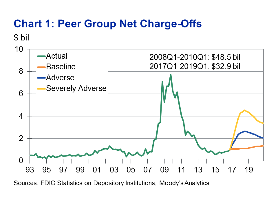
Determining when to charge off a loan is often an imprecise task, and the time required to recover on the loan can also be volatile. Therefore, we prefer to focus on net charge-offs accumulated over a period of time rather than a time series projection of quarterly charge-offs. We focus on a nine-quarter horizon to match that of the CCAR tests; our qualitative conclusions are unchanged if we use, for example, a four-quarter horizon.
We look at cumulative net charge-offs starting in the first quarter of 2017 for the CCAR scenarios, as performance over that nine-quarter CCAR window is of greatest current concern to banks. We use the second quarter of 2001 and the first quarter of 2008 as the starting quarters for the 2001 recession and Great Recession, respectively. Because charge-offs and recoveries tend to lag the general economy, an alternative approach would be to compare the worst (largest) nine-quarter cumulative net charge-offs in each economic cycle. That approach would result in larger losses, but the qualitative comparisons among recessions would be similar.
Chart 1 plots quarterly net charge-offs across all types of loans for the CCAR peer group. Table 2 summarizes our preferred nine-quarter cumulative net charge-off metric for the past two recessions and the three CCAR scenarios. In the Severely Adverse scenario, net charge-offs are about 32% lower than in the Great Recession, yet even that hides the much improved credit profile of the banks’ borrowers. During the Great Recession, banks’ cumulative net charge-offs totaled 4.1% of outstanding loans, while projected net charge-offs are only 2.7% under the renewed Severely Adverse scenario. Net charge-offs are slightly higher under the baseline than they were in the 2001 recession, but that is a result of loan portfolio growth: As a percentage of loans outstanding, net charge-offs are much lower in the current baseline. As a percentage of loans, net charge-offs in the Adverse scenario are slightly worse than those scenarios experienced during the 2001 recession.
| Table 2: Cumulative Net Charge-Offs of Peer Group | |||
| NCO | |||
| Event | $ bil | % | |
| 2001 recession | 9.7 | 1.24 | |
| Great Recession | 48.5 | 4.09 | |
| 2017 CCAR Baseline | 9.9 | 0.79 | |
| 2017 CCAR Adverse | 20.4 | 1.65 | |
| 2017 CCAR Severely Adverse | 32.9 | 2.69 | |
| Sources: FDIC Statistics on Depository Institutions, Moody’s Analytics | |||
Table 3 shows our forecasts of cumulative nine-quarter net charge-offs for the banks in the peer group under the Severely Adverse scenario. Only three of the banks are predicted to have higher net charge-offs than in the Great Recession. MUFG’s (Union Bank’s) increase is caused by a larger loan portfolio; as a percentage of loans outstanding, the bank’s net charge-offs actually decline significantly. Northern Trust’s loan portfolio represents a much smaller portion of its assets (27.2%) than the peer group as a whole (64.6%), so pinpointing the reason for its forecast increase in net charge-offs is more difficult.
| Table 3: Cumulative Net Charge-Offs for Selected Banks | ||||
| Great Recession | Severely Adverse Scenario | |||
| NCO, $ bil | NCO, % | NCO, $ bil | NCO, % | |
| BancWest Corp. | 1.4 | 3.27 | 0.9 | 1.52 |
| BB&T Corp. | 3.7 | 3.27 | 3.1 | 2.30 |
| BMO Financial Corp. | 5.1 | 6.34 | 3.6 | 6.29 |
| Citizens Financial Group Inc. | 4.0 | 3.66 | 3.6 | 3.58 |
| Comerica Inc. | 1.6 | 2.90 | 1.0 | 2.06 |
| Compass Bank | 1.8 | 4.13 | 1.7 | 2.87 |
| Fifth Third Bancorp | 5.9 | 6.80 | 2.8 | 2.99 |
| Huntington Bancshares Inc. | 3.2 | 5.16 | 1.5 | 2.27 |
| KeyCorp | 4.4 | 4.78 | 2.8 | 3.12 |
| M&T Bank Corp. | 1.3 | 1.52 | 1.2 | 1.41 |
| MUFG Americas Holdings Corp. | 1.8 | 3.43 | 2.1 | 2.72 |
| Northern Trust Corp. | 0.2 | 0.67 | 0.6 | 1.64 |
| Regions Financial Corp. | 4.5 | 4.65 | 2.5 | 3.10 |
| Santander Holdings USA Inc. | 1.9 | 3.27 | 3.3 | 6.63 |
| SunTrust Banks Inc. | 5.6 | 4.28 | 5.0 | 3.40 |
| Zions Bancorporation | 2.0 | 4.46 | 1.8 | 4.39 |
| Peer group | 48.5 | 4.09 | 32.9 | 2.69 |
| Industry | 342.5 | 4.36 | 267.7 | 2.94 |
| Sources: FDIC Statistics on Depository Institutions, Moody’s Analytics | ||||
Santander’s results are driven by a deterioration in its commercial and industrial portfolio (Chart 2). Over the course of 2016, Santander had net charge-offs of $126 million versus $59 million in 2015 and $49 million in 2014. Given the large jump in 2016 (despite benign economic conditions) we are not surprised that our forecasting algorithm foresees large losses should the Severely Adverse scenario occur.
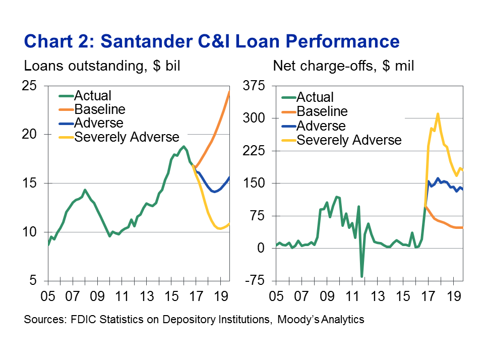
Table 4 breaks down loan performance for the largest categories of loans among the CCAR peer group[2]. Performance in percentage terms is better in the Severely Adverse scenario than the Great Recession for all categories. Consumer and credit card loans have relatively high net charge-off percentages because they are not directly backed by collateral. Nevertheless, as a share of balances, cumulative charge-offs are mild in the Severely Adverse scenario compared with prior recessions.
| Table 4: Peer Group Loan Performance | ||||
| Cumulative net charge-offs, % | ||||
| Loan category | 2001 recession | Great Recession | Severely Adverse Scenario | 2016Q4 balance, $ bil |
| Commercial and industrial | 2.62 | 3.37 | 2.57 | 366.1 |
| Residential 1-4 family first lien | 0.18 | 2.26 | 0.82 | 233.1 |
| Consumer | 2.68 | 4.57 | 3.05 | 143.9 |
| Home equity | 0.45 | 4.25 | 1.13 | 91.5 |
| Other consumer | 2.53 | 3.94 | 3.39 | 51.2 |
| Multifamily | 0.13 | 4.67 | 0.63 | 36.3 |
| Credit card | 9.82 | 18.43 | 10.48 | 12.3 |
| All | 1.24 | 4.09 | 2.69 | 1,242.1 |
| Sources: FDIC Statistics on Depository Institutions, Moody’s Analytics | ||||
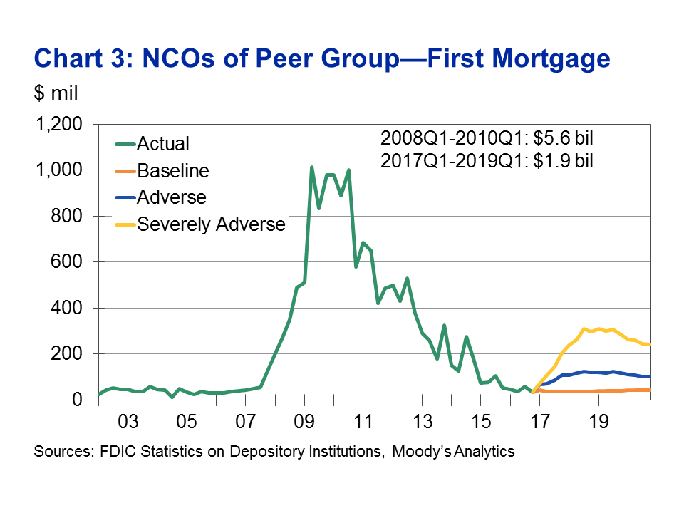
Credit quality in the residential housing sector has improved dramatically in the past decade, with higher down payments, increased documentation, and higher credit scores required for potential buyers to obtain mortgages. Chart 3 shows net charge-offs for first-lien residential mortgages for the peer group. Over the nine-quarter window starting in the first quarter of 2008, these 16 banks collectively wrote off more than $5.6 billion. In contrast, under today’s Severely Adverse scenario we predict charge-offs of a mere $1.9 billion.
Deposits
Although credit losses receive the bulk of the modeling attention at many banks, they are far from the only component necessary to carry out a complete stress test. A major advantage of the Bank CRF is that we have data for all items on banks’ financial statements. Industry-level forecasts combined with our peer group and bank-specific forecasting methodology allow us to produce a more complete picture of a bank’s financial health in various economic scenarios.
Chart 4 plots our forecasts for non-transaction account balances (including things such as money market accounts, certificates of deposit, and savings accounts) for the super-regional peer group. In general, these balances grow over time with little volatility. Nevertheless, a hint of the business cycle is evident in the data. During and immediately following the Great Recession, for example, balances dipped marginally and trended sideways. The Adverse and Severely Adverse forecasts therefore also reflect slight dips in the first half of the forecast horizon as household income growth slows. Later, these scenarios resume the established secular uptrend.

Even though deposit balances at the industry level and for large peer groups show little variation around the trend, movements at the bank level are more heterogeneous. For example, Chart 5 shows our forecasts for non-transaction account balances at Key Bank for the three CCAR scenarios. Given the broad uptrend in balances throughout most of the first decade of the 2000s, one might find our forecasts for flat balances to be too pessimistic. However, balances at Key Bank did decline throughout 2010 even as the recovery from the Great Recession took hold. Balances did not eclipse their prior peak until the second quarter of 2012. Moreover, while peer-group balances had moved sideways during the recession, they reverted to an upward trend by the end of 2010.

If an individual modeler at Key Bank built a regression model based on macroeconomic variables and came up with a tepid forecast, there might be some consternation and resistance from management. However, the CRF database allows us to investigate further and explain why this forecast is optimal. In Chart 6, we plot Key Bank’s non-transaction deposit balances as a share of the CCAR peer group’s balance. Key Bank’s market share had declined significantly from 2000 to 2007 despite a strong economy in the second half of that span. Its market share has again been declining since 2013. During the Great Recession and its aftermath, Key Bank’s market share recovered—the scenario forecasts of market share make sense given that history. When market share forecasts are combined with aggregate peer group forecasts, a full explanation of bank-level dynamics becomes clear.

Capital ratios
One of the goals of stress-testing is to determine whether banks have sufficient capital so that depositors and other creditors will not suffer losses if economic conditions deteriorate substantially. Here we focus on the tier-1 risk-based capital ratio, defined as tier-1 capital as a percentage of risk-weighted assets. Whether we use total tier-1 capital or common equity tier-1 capital, we would encounter the same types of challenges in the forecasting process that we describe below.
Capital ratios are among the hardest components of a stress test to forecast because they rely on many inputs and assumptions. Particularly at smaller and less complex institutions, quantitative modelers focus on forecasting credit losses and perhaps a few key pre-provision net revenue items. At larger institutions, they might also work on valuing securities and other holdings. To complete the capital plan, banks must consider whether they distribute capital in the form of dividends or stock buybacks and various legal fees and other expenses they might incur. Moreover, the banks must provide documentation supporting all their decisions.
Purely quantitative economic forecasts from the CRF can serve as a check on the bank’s subjective assumptions. Our forecasts are somewhat naïve—they are based on statistical, econometric models explaining how past capital decisions were made—but should nonetheless provide a useful benchmark for risk officers facing a difficult task. Our forecasts use the Moody’s Analytics structural economic macro forecast model which is updated monthly and accounts for more than 1,500 detailed economic variables.
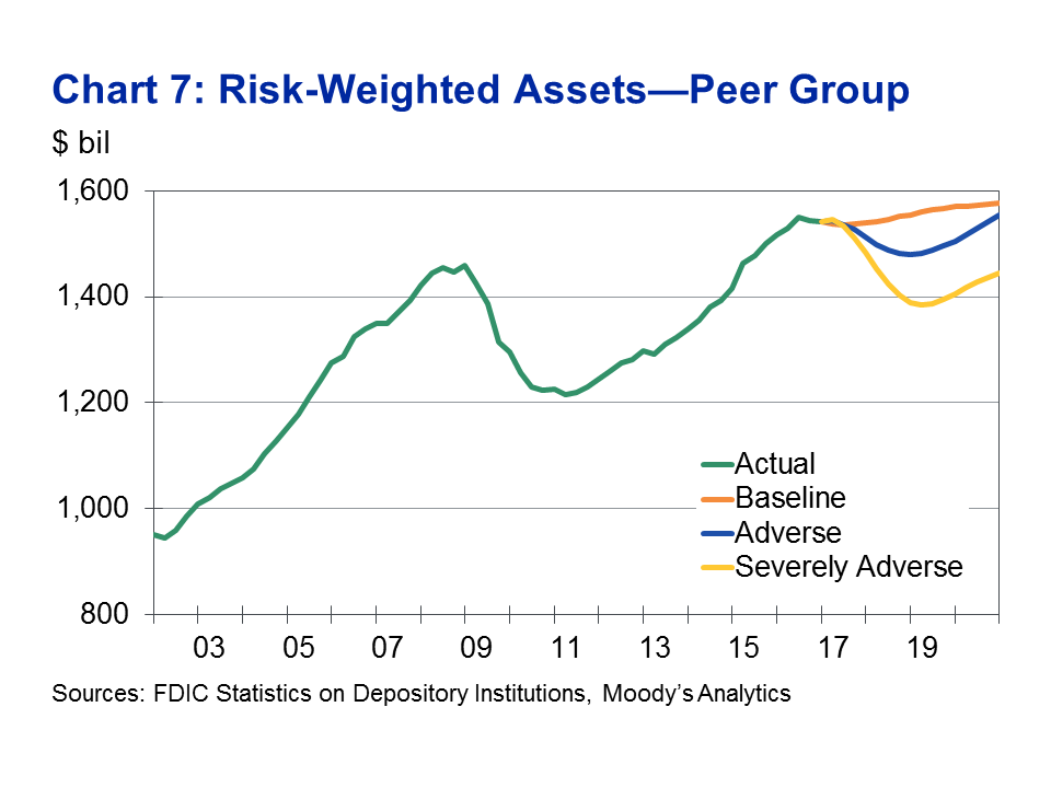
To forecast the tier-1 risk-based capital ratio, we forecast both tier-1 capital and risk-weighted assets under the various economic scenarios. To forecast RWA, we use the projections for banks and peer groups using the standard CRF algorithm. Regulatory and accounting changes over the years have changed how risk weights are assigned to various assets. Nevertheless, as Chart 7 shows, our forecasts of RWA for the peer group are plausible given the series’ historical behavior. Apart from a dip during the Great Recession, RWA has trended higher. RWA growth in the baseline appears tepid compared with growth early in the 2000s and from 2011 through 2015. However, Chart 8 shows that the peer group’s RWA as a share of the industry has been in secular decline since the early 2000s. Modest industry RWA growth combined with a declining market share explains this slow growth in RWA for the peer group. In the Severely Adverse scenario, RWA falls 10.2% against a 16.6% fall during the most recent recession.

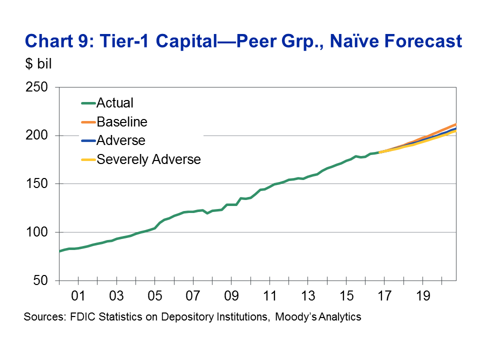
Forecasting tier-1 capital is more treacherous. Chart 9 shows a naïve forecast where our standard algorithm is applied to the historical series for the peer group. The series shows a remarkably steady upward trend, and the forecasts reflect this fact. Missing are the extraordinary measures taken by the government during the financial crisis to recapitalize foundering banks, particularly the Capital Purchase Program (CPP) within the larger Troubled Asset Relief Program (TARP). During late 2008 and 2009, the US Treasury invested more than $200 billion in 700 banks by purchasing preferred stock. Over the next several years, banks were able to repay and exit the program. From our perspective, the impact of the CPP was to make the observed tier-1 capital series much smoother than it would have been otherwise.
In this exercise, we therefore take a different approach to forecasting tier-1 capital. The change in capital from quarter to quarter is driven by three main items: net income, dividend payments, and stock sales and buybacks. One alternative is to assume that net stock transactions will be zero and that dividends are paid at the same rate as 2016, the last year of history. Chart 10 shows the peer group tier-1 capital forecasts using these alternative assumptions, and Chart 11 shows the resulting tier-1 capital ratios.
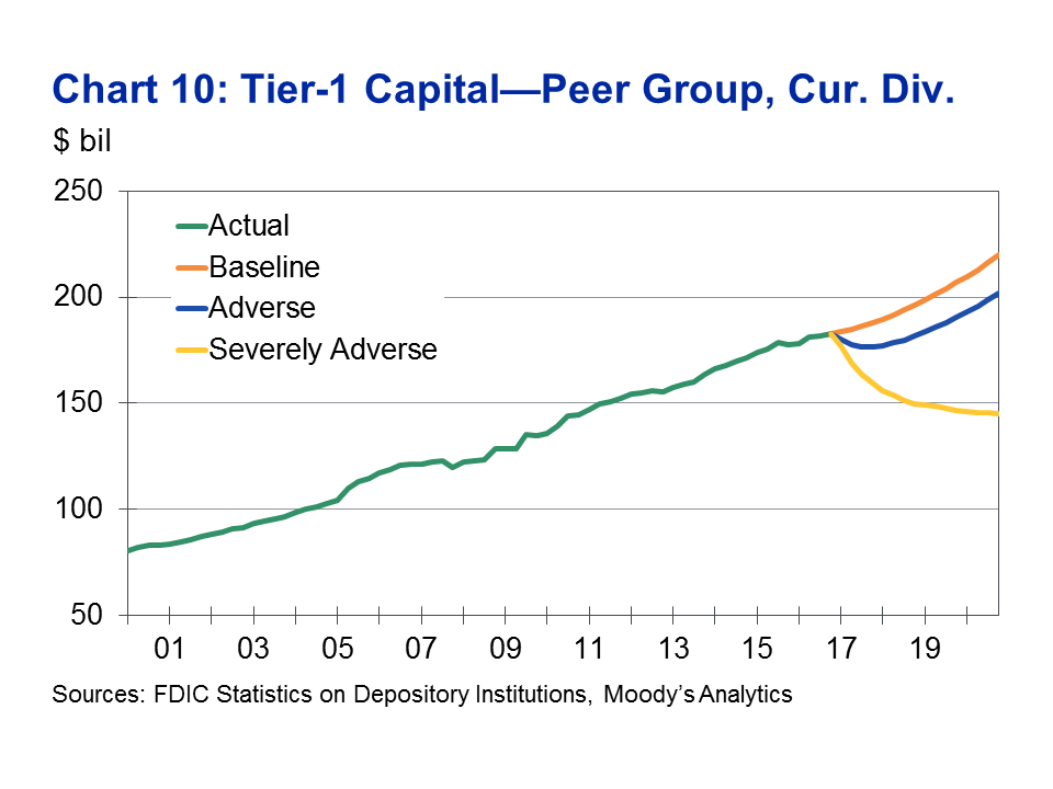

With the assumption that firms maintain current dividends, tier-1 capital in the baseline continues the trend from the past several years. The tier-1 capital ratio increases from its current 11.9% to 13.9% at the end of 2020 because capital is projected to increase more rapidly than RWA. In the Adverse scenario, tier-1 capital falls slightly through 2017 as net income declines, the economy weakens and net charge-offs rise. In this scenario, short-term rates stay near zero while the 10-year Treasury yield rises modestly, to 2.75% in the latter half of 2018. However, risk premia is assumed to increase more dramatically: mortgage rates exceed 5%, and Baa-rated corporate bonds rise to 6.5% by late 2017. These wide spreads promote improved bank profitability relative to the baseline.
In the Severely Adverse scenario, the peer group records nine-quarter losses, starting in the first quarter of 2017, of $7 billion, compared with $21.4 billion from the first quarter of 2008 through the first quarter of 2010. The peer group also pays dividends of $26.6 billion, assuming banks maintain 2016 dividends. Tier-1 capital falls more rapidly than RWA, so the tier-1 capital ratio falls to 10.8% in the first quarter of 2019 and 10.1% in the fourth quarter of 2020.
There are at least two shortcomings with the assumption that banks maintain current dividends. Dividend payments over the past five years have increased at a 15% annual rate, and under the baseline we have no reason to expect such dividend increases to dematerialize. The second regards the Severely Adverse scenario—in the face of higher credit losses, banks can reduce dividend payouts to preserve capital. This scenario is what happened during the financial crisis, and a realistic scenario would include similar dividend cuts again. One alternative would be to assume that dividend payouts are reduced to zero, but this assumption is not tenable. During the financial crisis, regulators soon realized that if all dividends were halted, investors with mandates that require dividends to be paid would be forced to divest. For the sake of this exercise, we therefore assume that dividend payments are cut in half. That fraction is arbitrary, though it does prevent a significant decline in the peer group’s projected tier-1 capital ratio.
Charts 12 and 13 show results under our preferred assumptions regarding capital distributions. Capital continues to accumulate in the baseline despite increasing dividend payments, though the capital ratio now ends 2020 at 13.2% versus the 13.9% seen with constant dividend payments. In the Severely Adverse scenario, tier-1 capital bottoms out in the third quarter of 2018 about $21 billion below its 2016 fourth quarter value. The capital ratio declines to 11.1% in the third quarter of 2017, lower than at any point since 2010 but still well above pre-financial crisis levels.


Methodology
Detailed descriptions of our approach and models are described in Hughes and Poi (2016)[3], Mehra (2016)[4], and Poi (2016)[5]. Here we provide a brief synopsis. To reiterate, we consistently apply the same approach for all concepts and all banks.
The CRF methodology is reductive in nature in the sense that we begin with aggregate industry data and identify macroeconomic forces that affect the entire banking system. We then isolate the trend and cycle from each bank’s market share, leaving us with series that reflect the bank’s own strategic decisions, the effects of its peers’ actions, and other idiosyncratic behavior. This two-layer approach to modeling allows us to disentangle macroeconomic and bank-specific effects. Peer groups can be viewed as an intermediate layer. Doing so allows us to differentiate between factors that affect the entire industry and factors that affect only the peer group of interest, whether because of geography, or because of particular portfolio concentrations[6].
For example, a bank runs a large marketing campaign for a particular product during a boom. One can reasonably assume that at least some of the observed increase in volume is the result of the marketing campaign rather than the state of the economy. Other peer banks that did not market themselves as aggressively will therefore not experience the same rate of growth. If the increased marketing is not merely a reflection of economic conditions, our methodology will find the aggressive bank’s market share growth to be idiosyncratic and will not extrapolate that growth through the forecast window.
Current approaches to PPNR modeling fail to draw these kinds of distinctions, assuming that all movements in the data are caused by external macroeconomic forces rather than internal manager-initiated actions. These approaches cannot be used to conduct “what-if” analyses that explore how management actions affect performance. In contrast, our forecasts provide a clear look at expected outcomes based on macro conditions, so that “what-if” analyses can focus on determining how management actions cause performance to deviate from the performance of the peer group.
Our primary modeling philosophy is one of humility. We recognize that it is difficult to identify, in one model, the myriad factors that contribute to the behavior of any single series being modeled, let alone an entire set of financial statements. We also recognize that building models of smooth series exhibiting clear cyclical behavior is generally more conducive to forecast accuracy than trying to correlate economic variables with noisy bank-level data.
Our approach therefore begins with fully specified industry-level econometric models for each series (see Mehra [2016]). Although the actions of an individual manager can have a profound impact on the behavior of the bank, these actions will have an undetectable impact on the industry as a whole. For this reason, we are safe in modeling the effect of macroeconomic variables on industry-level series without worrying about bank-specific management decisions.
One feature of our industry-level models is that they exploit adding-up constraints and identities that help anchor forecasts for noisier peripheral elements of the industry-level balance sheet and income statement. For example, we can understand the macroeconomic drivers of the total non-interest expense series better than we can for the subcategories that make up the series. We do construct models for each subcategory, but we adjust the forecasts so that they add up to the previously determined forecast for the smoother, more aggregate, series. The individual models for the subcategories help us distinguish the peculiarities of each series, while the more accurate forecasts of the smoother, broader series serve as guide rails.
We apply a similar “share down” process to project the behavior of individual banks. Many bank-level series are modeled using a market share approach, while for other series we use a “beta model” methodology analogous to well-known empirical explorations of the capital asset pricing model (see Poi [2016]). Our algorithms fit various market-share and beta models and use cross validation to pick the model that forecasts a particular series most accurately. A feature of the market share approach is that it prevents the modeler from forming prior expectations about the signs of macroeconomic factors’ coefficients. For example, although one can reasonably assume that industry-level mortgage credit losses will rise in a recession, one cannot say, a priori, whether Wells Fargo or Zions will have an increasing or decreasing share of such losses. Determining the effect of the macroeconomy on a bank’s market share for a series is thus a purely statistical exercise that does not require the modeler to justify the signs of any coefficients.
Our observation that banks’ market shares often exhibit trend behavior typically yields few objections. Our claim that market shares are often pro- or countercyclical is somewhat more controversial. Charts 14 and 15 show the market shares of commercial and industrial loan balances for some of the banks in our peer group. Chart 14 shows Comerica, M&T, MUFG, and Compass, all of which have market shares that exhibit predominantly trending behavior. None of these market shares exhibit much relationship to the macroeconomic cycle, so share forecasts show little deviation between the baseline, Adverse and Severely Adverse scenarios [7].
In contrast, the market shares shown in Chart 15 display clear correlation to the macroeconomy. During the Great Recession, BB&T increased its share and then cut back as the recovery took hold. Santander increased its market share in the expansion before the Great Recession and then reduced its exposure during the event. Huntington clearly gained traction during the downturn. The dynamics of Fifth Third’s market share are more difficult to discern, but there is a strong cyclical component as evidenced by the different trajectories for market share under the various scenarios. Cyclical changes in market share might reflect conscious decisions made by bank managers or passivity in the face of rivals’ aggression. We typically find that conservative banks have countercyclical market share in most asset categories. Procyclicality is often allied to an upward trend in market presence, reflecting the fact that such banks are taking risks to gain an increased share.
Poi (2016) describes in detail how we use principal components analysis to control for the effects of the economy when fitting a bank’s or peer group’s market share or beta model. Researchers at the Federal Reserve have advocated the use of principal components and similar methods to control for macroeconomic variables (see, for example, Groen and Kapetanios [2015][8]). One shortcoming of the technique is that interpretation of the principal components is often non-intuitive. Poi (2016) nevertheless shows that of the three principal components we consider, the first is clearly a reflection of blended short- and long-term interest rates over time. The other two components reflect the ebbs and flows of the business cycle, particularly various employment and output measures. Together, the three principal components account for nearly 85% of the variation seen in about 50 key financial, macroeconomic, and interest-rate variables.
Conclusion
The super-regional CCAR banks appear to be in a safe position. Capital cushions are either sufficient or excessive and the potential for extreme credit losses appears low. This position is not surprising given the regulatory scrutiny applied to the banks since the recession. Lending standards have been sound or tight in most areas and there appear to be no significant lending bubbles to threaten the structural stability of the banking system. It will be interesting to see whether the conclusion of the 2017 stress-test process, due to be published in coming weeks, agrees with our findings.
We suspect, however, that the Fed’s results will be substantially more pessimistic than ours. Bank examiners, for good reason, have a strong tendency to be biased in favor of conservatism and will thus apply their thumb to the scale to ensure that bank capital levels are at least slightly excessive. Though this bias is justified, it leaves a significant hole in our (and their) understanding of the banking system. With this approach, neither the public, nor the banks, are presented with a detailed, unbiased financial projection for the behavior of the entire system.
[1] Fed officials make this directive explicit in their documentation: “Given the uncertainty inherent in a forward-looking capital planning exercise, the Federal Reserve expects BHCs to apply generally conservative assumptions throughout the stress-testing process to ensure appropriate tests of the BHCs' resilience to stressful conditions.” Taken from “Capital Planning at Large Bank Holding Companies: Supervisory Expectations and Range of Current Practice,” which is available online.
[2] Owner-occupied commercial real estate loans and other non-residential real estate loans are also large categories, with peer group assetsof $91.3 billion and $86.1 billion as of the fourth quarter of 2016, respectively, but they were not added to the call reports until 2007, so we have excluded them from this table.
[3]A.Hughes and B. Poi, “Stress-Testing and Strategic Planning Using Peer Analysis,” Risk Perspectives, Vol. 8 (November 2016): 59-68.
[4]S.Mehra, Bank Call Report Forecast Database, Moody’s Analytics product literature (2016).
[5] B. Poi, Peer-Group Analysis in Bank Call Report Forecasts, Moody’s Analytics product literature (2016).
[6] Bank-level forecasts will thus depend on the set of peers chosen. This dependency can be avoided by using an industry-level peer group. In our view, however, the peer group layer provides a strong signal, especially if the peer group is carefully chosen.
[7] Note that since the industry forecasts exhibit significant stress, all four banks will be projected to suffer under the Severely Adverse scenario.
[8] Jan J.J. Groen and G. Kapetanios, “Revisiting Useful Approaches to Data-Rich Macroeconomic Forecasting,” Federal Reserve Bank of New York Staff Report #327 (May 2008, revised October 2015).